The Forecasting Problem Nobody Warns You About
If you sell direct-to-consumer, your sales data probably looks pretty clean. Orders come in every day, there's a weekly rhythm where weekdays outperform weekends, an annual pattern where November spikes and January dips, and a growth trend you can eyeball. Forecasting this should be straightforward, right?
It's more complicated than it looks. Those weekly and yearly patterns interact with each other in ways that trip up a lot of models. A Monday in November does not behave the same as a Monday in February, and models that handle one seasonal cycle well often struggle when two cycles overlap. On top of that, growth is rarely linear. A brand might grow steadily for 18 months and then accelerate or plateau, and the model needs to detect when that trajectory shifts. Add in irregular holiday effects like Black Friday moving every year or shipping cutoff deadlines creating artificial demand cliffs in December, and things get messy fast.
Then there's the problem of sudden shocks. A product goes viral on social media and demand surges for 72 hours. Most forecasting models treat that spike as noise and smooth right over it, which means your inventory plan misses the moment entirely.
Another problem I found while researching is that most D2C brands don't just sell direct, they also sell wholesale. Wholesale demand behaves nothing like D2C. Most days have zero B2B sales, and then out of nowhere, a retailer places an order for 1,500 units. There is no weekly pattern, no smooth trend. Just long stretches of nothing punctuated by large, irregular orders.
D2C and B2B are fundamentally different statistical problems. Trying to force both into a single model is a mistake. They need separate forecasting strategies, and then you combine the results into one inventory plan.
The Project: Multi-Channel Forecasting for Nomatic
I built a forecasting dashboard around this problem using Nomatic as the case study. Nomatic is a premium travel bag and gear brand that sells both D2C through their own site and B2B through wholesale partnerships with retailers. That dual-channel structure makes them a perfect example of why one forecasting approach can't cover everything.
I picked Nomatic for this because I really like the brand, and it is local to Utah. I love what they have done and think they do amazing work (hey if you need a data analyst @Nomatic, hire me).
The data is synthetic. I generated three years of daily sales data that mirrors the patterns a multi-channel brand like Nomatic would show, so I could focus on methodology without needing proprietary data. The dashboard itself produces a 6-month inventory recommendation that combines both channels, with explicit risk trade-offs so you can choose how much safety stock to carry.
I'll walk through the D2C side first (where I used tools I was already comfortable with), then the B2B side (where I was less experienced), and then what the industry is doing now to push forecasting further.
The D2C Side: Tools I Already Knew
D2C data is what most people picture when they think about sales forecasting. Sales every single day for three years, a clear weekly pattern where weekdays sell about 33% more than weekends, a clear annual pattern with holiday spikes and summer travel bumps, and steady upward growth from roughly 125 units per day to 185 units per day over the three-year period. This is the easier side of the forecasting problem.
I came into this project already familiar with the main tools for this kind of data, so the D2C side was about picking the right one rather than learning something new.
ARIMA and SARIMA are the classic statistical approach. They work well for short-term forecasts where recent momentum dominates, but they're brittle with missing data and require you to explicitly parameterize each seasonal cycle. If you have both weekly and yearly seasonality interacting, the configuration gets complex fast and it's easy to get wrong.
Exponential Smoothing (ETS/Holt-Winters) is computationally lightweight and handles a trend plus one seasonal period well, but like ARIMA, it starts to struggle when you need to model weekly and yearly seasonality simultaneously. There are extensions like TBATS that help with multiple seasonalities, but at that point you're adding a lot of complexity to a model that was attractive because it was simple.
Facebook Prophet takes a different approach entirely. Instead of autoregression, it treats forecasting as curve-fitting and decomposes the time series into trend, weekly seasonality, and yearly seasonality, then sums them. It handles multiple seasonalities natively, is robust to missing data, and produces uncertainty intervals out of the box. The tradeoff is that it tends to over-smooth sudden short-term shocks because it treats them as noise rather than signal, so if you're in a space where viral moments drive a big chunk of your sales, Prophet might not react fast enough.
Amazon Chronos is the newest entrant in this space. Released in 2024, Chronos is a foundation model for time series built on transformer architecture. The big difference from Prophet is that Chronos can do zero-shot forecasting using pre-trained weights from diverse time series datasets, so you don't necessarily need to train it on your specific historical data. It's a different paradigm, more like using a pre-trained language model versus writing your own rules, and it's worth keeping an eye on as the approach matures.
Personally, my favorite of these tools is Prophet. Mainly because it is so simple to use in R, and for me it has been great to quickly get an idea of the trajectory of a stock, company performance, or even patient demand in healthcare.
In this project my favorite method also ended up being the best fit. D2C sales had strong dual seasonality and a multi-year growth trend, which is exactly what Prophet is designed for. I trained the model on years one and two, then tested it on year three. The backtest produced a MAPE of 13.3%, meaning the forecast was off by about 13% on average. In demand forecasting, under 20% MAPE is generally considered good and under 10% is excellent, so this lands in solid territory. The 6-month forward forecast projects roughly 28,474 D2C units.
The B2B Problem: When Most Days Are Zeros
Everything I just described works because D2C data is continuous. The B2B side breaks all of it.
Out of 1,095 days of B2B data, only 101 had any sales at all, which is a 9.2% activity rate. When orders did come they averaged 884 units, with individual orders ranging from 200 to 2,500 units. There's no weekly rhythm, no smooth growth curve, just sporadic large orders separated by long stretches of nothing.
If you apply a standard forecasting model to this data, you get what I'd describe as a "drizzle" forecast. The model averages the sparse orders across all days and predicts a small fractional amount every single day. That prediction is mathematically defensible and completely useless for actual inventory planning. You don't need 8 units today, every day, for six months. You need zero units most days and then suddenly 1,200 units on a Tuesday in March.
This type of data is called intermittent demand, sometimes lumpy demand in supply chain terminology. It's common in wholesale, spare parts, and specialty manufacturing. It turns out there's an entire family of forecasting methods built specifically for this problem, and I had no idea it existed before I started researching for this project. I should have guessed that there were already solid techniques out there. I keep finding that the book has already been written and I just need to learn from it, the creativity on my end is all about how to apply those models in new or better ways.
What I Learned About Intermittent Demand
When I started digging into how the supply chain world handles intermittent demand, I found a progression of methods I'd never encountered before.
Croston's Method and Its Successors
Croston's Method (1972) was the first major innovation for this problem. Instead of trying to forecast demand directly, it splits the problem into two components: the size of demand when it occurs, and the interval between demand events. It tracks each separately using exponential smoothing and divides the smoothed size by the smoothed interval to get a forecast rate. This was a smart idea for its time, but it has a critical flaw. Croston's only updates its estimates when a positive demand event occurs. If a wholesale partner stops ordering, the model never notices and keeps forecasting demand for a product or channel that has gone dead. A later refinement called the Syntetos-Boylan Approximation (SBA) added a bias correction to fix Croston's tendency to over-forecast, but it inherited the same structural problem: silence from a customer looks the same as "we just haven't ordered yet."
TSB: Solving the Obsolescence Problem
The Teunter-Syntetos-Babai method (TSB, 2011) takes a fundamentally different approach. Instead of tracking inter-demand intervals, it tracks demand probability directly, and critically, it updates that probability every single period whether demand occurs or not. When a day passes with no order, the probability decays exponentially. So if a wholesale partner churns, the forecast gracefully trends toward zero instead of stubbornly predicting future demand that will never come.
TSB solves the theoretical problem elegantly, but it still produces a single point forecast. For B2B inventory planning where individual orders can swing by thousands of units, a single number isn't enough. You need to understand the full range of possible outcomes.
Building a Monte Carlo Approach with the Right Distribution
I was already familiar with Monte Carlo simulation from other work. I used it for budget simulation in a healthcare case competition to model potential cost fluctuations, so the general idea of running thousands of scenarios and looking at the distribution of outcomes wasn't new to me. But applying it to supply chain inventory planning was new territory, and the process of figuring out the right inputs taught me just as much as the results did.
The first step was proving that B2B orders cluster at quarter-ends. A two-proportion Z-test showed that the spike rate during the last 15 days of each quarter was 17.8%, compared to 7.5% during the rest of the year (Z = 4.44, p < 0.00001). Retailers genuinely tend to restock at quarter-ends, and this confirmed it statistically rather than just eyeballing the pattern.
The second step was modeling spike sizes, and this is where I hit something I didn't expect. I initially assumed I could model order sizes with a normal distribution, but it just didn't work. The data is right-skewed and strictly positive, with most orders falling in the 200 to 800 unit range but a long tail reaching up to 2,500. A log-normal distribution turned out to be the right fit, which I validated using a Kolmogorov-Smirnov (KS) test (p = 0.52, well above the 0.05 threshold). The KS test was another tool I hadn't used before. It measures how well a theoretical distribution matches observed data by comparing their cumulative distributions, and it was really helpful for confirming that my distributional assumption wasn't just wishful thinking.
With those pieces in place, I ran 1,000 Monte Carlo simulations of 180-day periods. Each simulation randomly determined whether each day had an order (using the higher 17.8% probability for quarter-end days and 7.5% otherwise), and if so, drew the order size from the fitted log-normal distribution. The results gave me the range I needed:
- P10 (~9,551 units): the optimistic scenario, only 10% of simulations were lower
- P50 (~14,437 units): the expected level, the median outcome
- P90 (~20,062 units): the safety planning level, covers 90% of possible outcomes
This also led me to learn about P-quantile safety stock. Traditional safety stock formulas use a Z-score multiplied by standard deviation, which assumes demand follows a normal distribution. When demand is actually log-normal like this B2B data, that formula can miscalculate your buffer by a pretty wide margin. Extracting percentiles directly from the Monte Carlo simulation is distribution-agnostic, it doesn't care what shape the data takes, it just gives you the actual P90 from the simulated outcomes. If I had just defaulted to the standard formula without thinking about it, I would have gotten the wrong answer for this data.
Combining Both Channels into One Inventory Plan
The final step was combining Prophet's D2C forecast with the Monte Carlo B2B projections into a single month-by-month inventory recommendation.
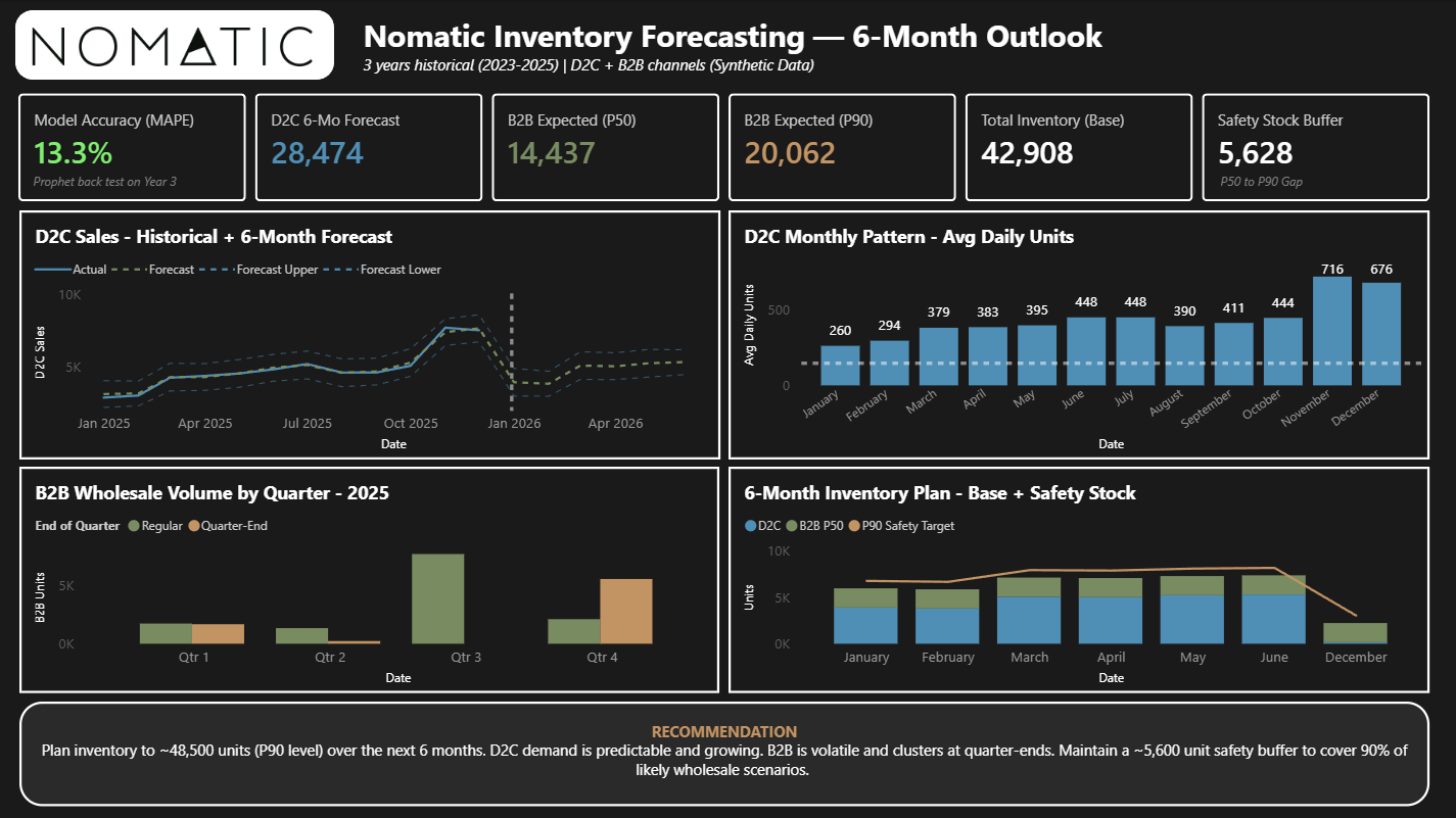
The dashboard presents two scenarios. The base plan (D2C forecast + B2B P50) totals roughly 42,900 units over six months, which is capital-efficient but accepts the risk of stockouts if wholesale orders come in heavier than expected. The safety plan (D2C forecast + B2B P90) totals roughly 48,500 units. The gap between the two, about 5,600 units, is the safety stock buffer, and that's basically the cost of covering 90% of possible wholesale scenarios.
What I really took away from this part of the project is that the question isn't "how many units will we sell?" It's more like "how many units should we have on hand, given how unpredictable the B2B channel is?" The model gives you a range and a trade-off, not a single answer. Whether a company like Nomatic should stock to P50 or P90 depends on their margins, their storage costs, and how much damage a missed wholesale order does to that relationship.
What the Industry Is Doing Now
The methods I used in this project are established and well-understood. The industry is already pushing beyond them in a few directions that I found really interesting while doing research for this project.
Virtual Pooling replaces the common practice of partitioning inventory by channel, where you might have a fixed allocation for Amazon, another for wholesale, and another for D2C. Instead, all inventory sits in a single shared pool and is dynamically allocated through real-time Available-To-Promise (ATP) calculations. This solves a problem I hadn't really thought about before: a brand could sell out of D2C inventory while identical units sit on a wholesale pallet in the same warehouse, just because they were allocated to a different channel.
ML integration adds exogenous variables that historical sales data alone can't capture. Tree-based models like XGBoost and deep learning approaches like LSTMs can ingest macroeconomic indicators, competitor pricing, social sentiment, and wholesale partner inventory depletion reports. The goal isn't to replace statistical methods but to combine them with models that pick up on external signals the historical data doesn't contain.
Daily parameter recalibration addresses something I noticed about my own model: the Monte Carlo uses fixed historical probabilities that never change. In a production system, those probabilities would be recalibrated daily using live data feeds so the model adapts when conditions shift. If a new wholesale partner comes on or an existing one churns, the model should pick that up in real time rather than waiting for someone to retrain it.
What I built is definitely not the end goal. This would be a first iteration for a smaller company as they gathered more data, improved their pipelines, and over time you could get more and more accurate with these methods layered on top.
Closing Thoughts
The D2C side of this project was familiar territory. Prophet, ARIMA, exponential smoothing. I came in knowing those tools and when to reach for each one. The B2B side was just so new to me. Intermittent demand was a whole problem class I didn't know existed, with its own family of methods stretching back to the 1970s. Learning that log-normal distributions were necessary (not just convenient), discovering the KS test for validating that fit, and understanding why P-quantile safety stock is more reliable than the standard Z-score formula on non-normal data were all genuine discoveries for me.
Even though the data I used was made up, these are real workflows that a D2C company could use. If you made it this far, I hope that you also learned something and maybe found ways to take it that next step with ML models like XGBoost to improve forecasting accuracy. I am hoping to revisit this and integrate those as well so I can see how these models are used in D2C contexts.
Thanks for reading.
Sources
- Croston, J.D. (1972). Forecasting and stock control for intermittent demands. Operational Research Quarterly, 23(3), 289-303.
- Taylor, S.J. & Letham, B. (2018). Forecasting at scale. The American Statistician, 72(1), 37-45.
- Ansari, A.F., Stella, L., Turkmen, C., et al. (2024). Chronos: Learning the language of time series. Amazon Science.
- Teunter, R.H., Syntetos, A.A., & Babai, M.Z. (2011). Intermittent demand: Linking forecasting to inventory obsolescence. European Journal of Operational Research, 214(3), 606-615.
- Syntetos, A.A. & Boylan, J.E. (2005). The accuracy of intermittent demand estimates. International Journal of Forecasting, 21(2), 303-314.